Protein-Ligand Contacts
Overview
DynamiSpectra offers a robust analytical framework to quantify the number of contacts between protein and ligand throughout molecular dynamics simulations, utilizing input data in .xvg file format. This analysis facilitates a detailed characterization of intermolecular interactions and binding dynamics.
The software’s graphical interface enables the visualization of the average number of contacts calculated across multiple simulation replicates, with the associated standard deviation represented as a shaded region illustrating variability. Furthermore, DynamiSpectra accommodates the analysis of individual simulation replicas, allowing users to generate plots from a single dataset when multiple replicas are unavailable or unnecessary.
Command line in GROMACS to generate .xvg files for the analysis:
gmx mindist -f Simulation.xtc -s Simulation.tpr -n index.ndx -on Contacts.xvg -d 0.35
def contact_analysis(output_folder, *simulation_file_groups, contact_config=None, density_config=None)
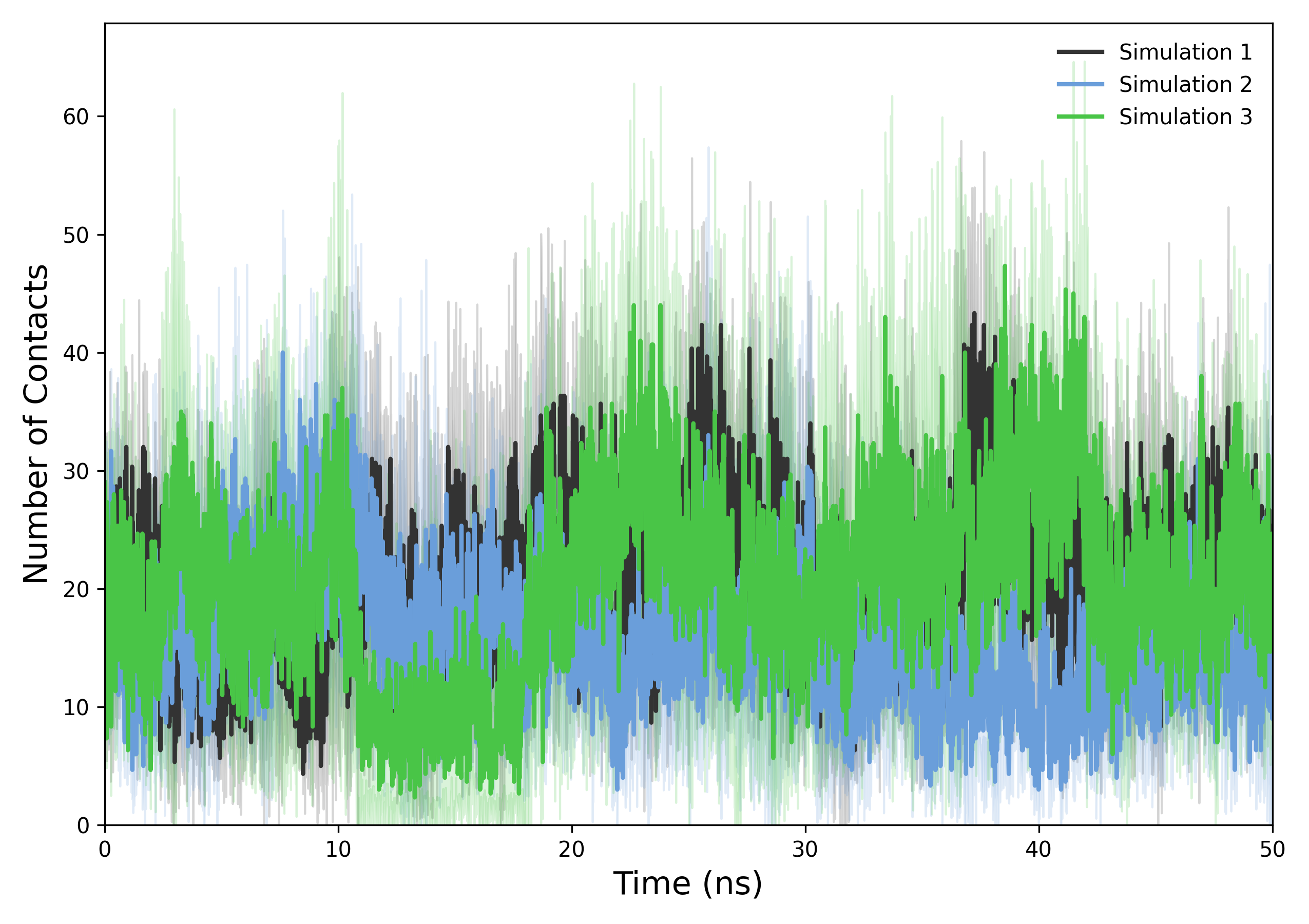
Interpretation guidance: The resulting plots depict the temporal evolution of protein-ligand contacts. A stable profile suggests persistent interactions and binding stability, whereas notable deviations may indicate conformational changes, ligand dissociation events, or alternative binding modes.
def plot_contact_density(results, output_folder, config=None)
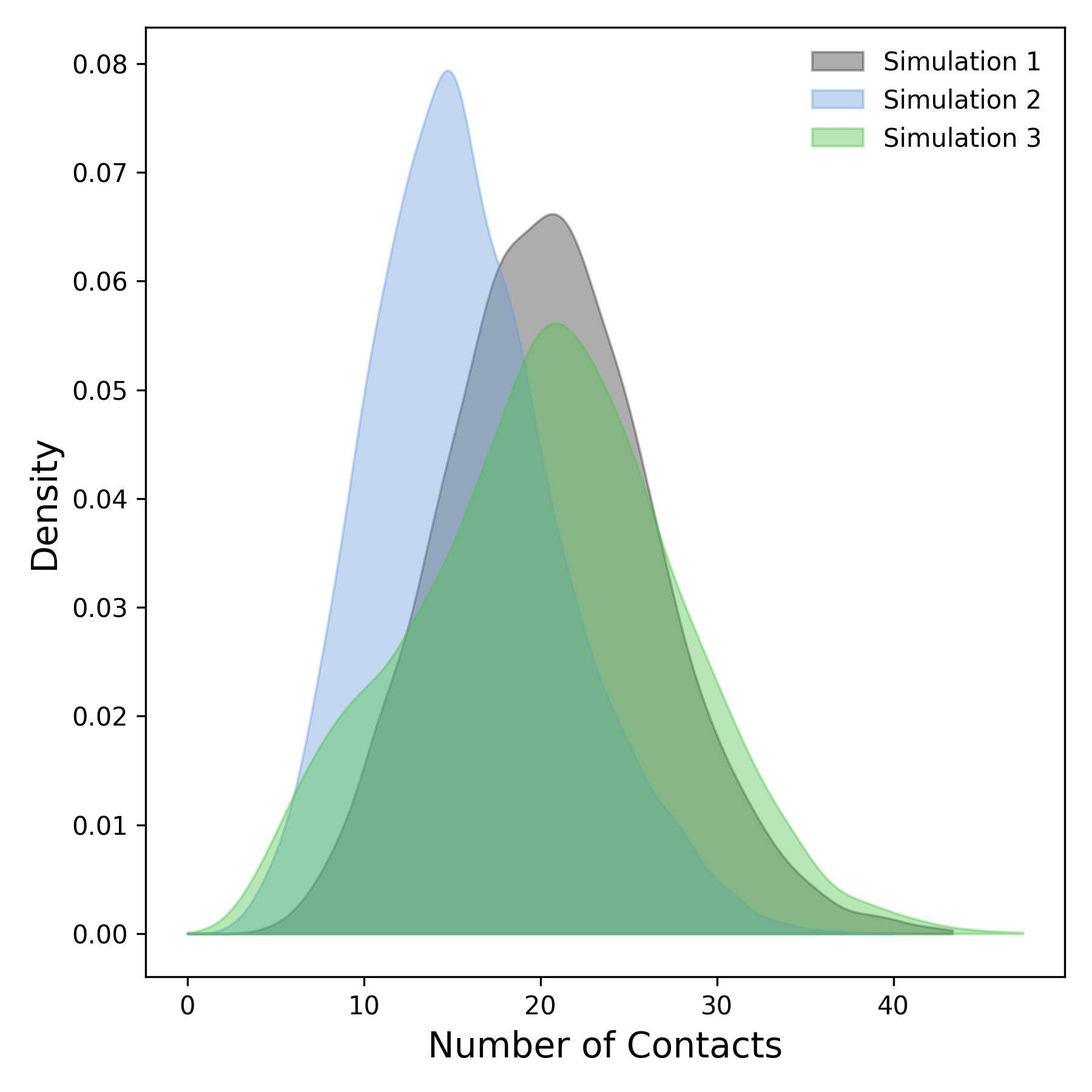
Interpretation guidance: This plot depicts the density distribution derived from the temporal profile of protein-ligand contacts. Peaks in the distribution correspond to regions exhibiting a higher frequency of interactions. Broader peaks indicate a more heterogeneous or variable contact pattern, while sharper, more pronounced peaks reflect stable and well-defined interaction regions between the protein and ligand.
Complete code
import numpy as np
import matplotlib.pyplot as plt
from scipy.stats import gaussian_kde
import os
def read_contacts(file):
"""
Reads contact data from a .xvg file.
Skips header lines and extracts time (in ns) and contact values.

Parameters:
-----------
file : str
    Path to the .xvg file

Returns:
--------
times : np.ndarray
    Array of time points in nanoseconds.
contacts : np.ndarray
    Array of contact counts at each time point.
"""
try:
    times = []
    contacts = []
    with open(file, 'r') as f:
        for line in f:
            # Skip metadata or comment lines (start with #, @, or ;)
            if line.startswith(('#', '@', ';')) or line.strip() == '':
                continue
            try:
                values = line.split()
                if len(values) >= 2:
                    time_ps, contact_val = map(float, values[:2])
                    times.append(time_ps / 1000.0)  # Convert from picoseconds to nanoseconds
                    contacts.append(contact_val)
            except ValueError:
                # If conversion to float fails, skip the line
                continue

    # Check if any valid data was read
    if len(times) == 0 or len(contacts) == 0:
        raise ValueError(f"File {file} does not contain valid data.")

    return np.array(times), np.array(contacts)

except Exception as e:
    # Print error if something goes wrong while reading the file
    print(f"Error reading file {file}: {e}")
    return None, None
def check_simulation_times(*time_arrays):
"""
Checks if all simulation time arrays are consistent (equal).
Raises an error if times do not match to avoid misaligned averaging.
"""
for i in range(1, len(time_arrays)):
    # Compare current time array with the first one
    if not np.allclose(time_arrays[0], time_arrays[i]):
        raise ValueError(f"Simulation times do not match between file 1 and file {i+1}")
def plot_contacts(results, output_folder, config=None):
"""
Plots the mean number of contacts over time with shaded std deviation.

Parameters:
-----------
results : list of tuples
    Each tuple is (time_array, mean_contacts, std_contacts) for one simulation group.
output_folder : str
    Folder path to save the plots.
config : dict, optional
    Plot configuration dictionary (colors, labels, axis labels, etc.)
"""
plt.figure(figsize=config.get('figsize', (9, 6)))

# Plot mean ± std for each simulation group
for idx, (time, mean, std) in enumerate(results):
    label = config['labels'][idx] if config and 'labels' in config else f'Simulation {idx+1}'
    color = config['colors'][idx] if config and 'colors' in config else None
    alpha = config.get('alpha', 0.2)

    # Plot average contact line
    plt.plot(time, mean, label=label, color=color, linewidth=2)

    # Plot shaded region for standard deviation
    plt.fill_between(time, mean - std, mean + std, color=color, alpha=alpha)

# Axis labels and formatting
plt.xlabel(config.get('xlabel', 'Time (ns)'), fontsize=config.get('label_fontsize', 12))
plt.ylabel(config.get('ylabel', 'Number of Contacts'), fontsize=config.get('label_fontsize', 12))
plt.legend(frameon=False, loc='upper right', fontsize=10)
plt.tick_params(axis='both', which='major', labelsize=10)

# Dynamically adjust axis limits based on data
max_time = max([np.max(time) for time, _, _ in results])
max_val = max([np.max(mean + std) for _, mean, std in results])
plt.xlim(0, max_time)
plt.ylim(0, max_val * 1.05)  # Add 5% margin above max value

plt.tight_layout()

# Create output folder if it doesn't exist
os.makedirs(output_folder, exist_ok=True)

# Save plots in TIFF and PNG formats
plt.savefig(os.path.join(output_folder, 'contacts_plot.tiff'), dpi=300)
plt.savefig(os.path.join(output_folder, 'contacts_plot.png'), dpi=300)

plt.show()
def plot_contact_density(results, output_folder, config=None):
"""
Plots kernel density estimates of the contact number distributions.

Parameters:
-----------
results : list of tuples
    Each tuple is (time_array, mean_contacts, std_contacts).
    Only the mean_contacts array is used here for density estimation.
output_folder : str
    Folder path to save the density plots.
config : dict, optional
    Plot configuration dictionary.
"""
plt.figure(figsize=config.get('figsize', (6, 6)))

# Plot KDE for each simulation group's mean contact values
for idx, (_, mean, _) in enumerate(results):
    kde = gaussian_kde(mean)  # Perform KDE on mean contacts
    x_vals = np.linspace(0, max(mean), 1000)  # Range for plotting KDE

    label = config['labels'][idx] if config and 'labels' in config else f'Simulation {idx+1}'
    color = config['colors'][idx] if config and 'colors' in config else None
    alpha = config.get('alpha', 0.5)

    # Plot KDE curve as a filled area
    plt.fill_between(x_vals, kde(x_vals), color=color, alpha=alpha, label=label)

# Axis labels and formatting
plt.xlabel(config.get('xlabel', 'Number of Contacts'), fontsize=config.get('label_fontsize', 12))
plt.ylabel(config.get('ylabel', 'Density'), fontsize=config.get('label_fontsize', 12))
plt.legend(frameon=False, loc='upper right', fontsize=10)
plt.tight_layout()

# Save density plots
plt.savefig(os.path.join(output_folder, 'contacts_density.tiff'), dpi=300)
plt.savefig(os.path.join(output_folder, 'contacts_density.png'), dpi=300)

plt.show()
def contact_analysis(output_folder, *simulation_file_groups, contact_config=None, density_config=None):
"""
Main function to process multiple simulation groups and generate plots.

Parameters:
-----------
output_folder : str
    Directory where the plots will be saved.
*simulation_file_groups : list of lists
    Each element is a list of file paths for replicates of a simulation group.
contact_config : dict, optional
    Configuration for the contact vs time plot.
density_config : dict, optional
    Configuration for the density plot.
"""
def process_group(file_paths):
    # Read time and contact data from all replicas in the group
    times = []
    contacts = []
    for file in file_paths:
        time, contact_val = read_contacts(file)
        times.append(time)
        contacts.append(contact_val)

    # Ensure all replicas are aligned in time
    check_simulation_times(*times)

    # Compute mean and std across replicas
    mean_contacts = np.mean(contacts, axis=0)
    std_contacts = np.std(contacts, axis=0)
    return times[0], mean_contacts, std_contacts

results = []
for group in simulation_file_groups:
    if group:
        # Process each simulation group (set of replicas)
        time, mean, std = process_group(group)
        results.append((time, mean, std))

# If at least one group is processed, generate plots
if len(results) >= 1:
    plot_contacts(results, output_folder, config=contact_config)
    plot_contact_density(results, output_folder, config=density_config)
else:
    raise ValueError("At least one simulation group is required.")