Protein–Ligand Hydrophobic Contacts
Overview
DynamiSpectra offers a robust and versatile analytical framework designed to quantify and monitor hydrophobic contacts between protein and ligand molecules throughout molecular dynamics simulations. Utilizing input data in standardized .xvg file format, this module enables researchers to characterize the extent and dynamics of hydrophobic interactions, which are fundamental for molecular recognition, binding affinity, and complex stability.
This analysis provides detailed insights into the temporal evolution of hydrophobic contacts, allowing identification of transient contacts, persistent hydrophobic patches, or disruption of interactions. By incorporating data from multiple simulation replicates, DynamiSpectra computes averaged contact profiles with corresponding variability measures, such as standard deviation, facilitating statistically meaningful interpretation. Moreover, the software supports analysis of individual simulation replicas, enabling flexible usage when replicate data are unavailable or unnecessary.
Command line in GROMACS to generate .xvg files for the analysis:
gmx select -f Simulation.xtc -s Simulation.tpr -n index.ndx -select 'group "LIG" and within 0.6 of (resname ALA VAL LEU ILE PHE MET and group "Protein")' -os Hydrophobic_contacts.xvg
def hydrophobic_analysis(output_folder, *simulation_file_groups, contact_config=None, density_config=None)
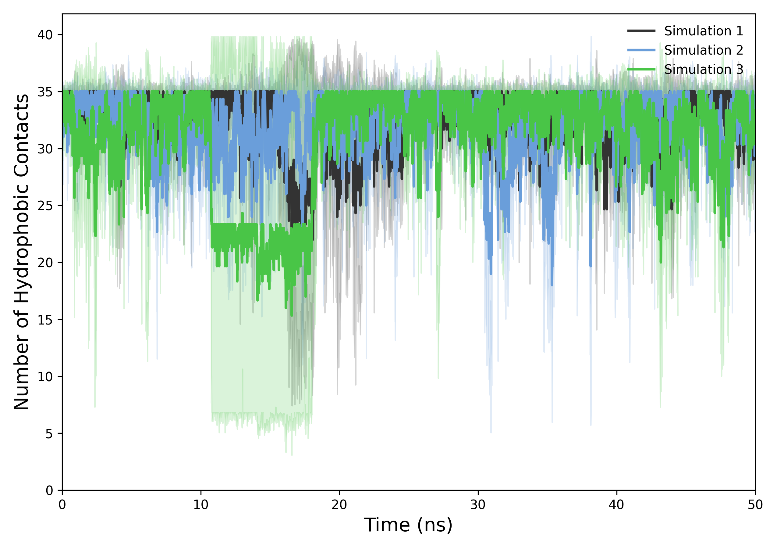
Interpretation guidance: The resulting plots illustrate the temporal progression of hydrophobic contacts between protein and ligand. A consistently high number of contacts indicates stable hydrophobic interactions and sustained binding affinity, whereas notable decreases or fluctuations may reflect conformational changes, disruption of hydrophobic patches, or transient binding events.
def plot_contact_density(results, output_folder, config=None)
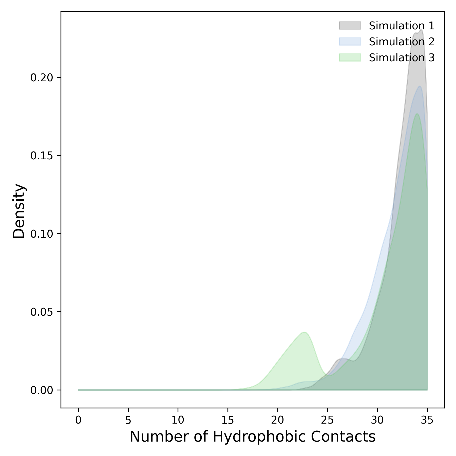
Interpretation guidance: This plot represents the density distribution derived from the temporal profile of minimal distances between protein and ligand. Peaks in the distribution indicate preferred interaction distances that occur more frequently during the simulation. Broader peaks suggest a more heterogeneous and variable range of distances, whereas sharper and well-defined peaks reflect stable and consistent spatial proximities maintained throughout the simulation.
Complete code
import numpy as np
import matplotlib.pyplot as plt
import os
from scipy.stats import gaussian_kde
def read_contacts(file):
"""
Reads a .xvg file containing hydrophobic contacts over time.

Parameters:
-----------
file : str
    Path to the .xvg file.

Returns:
--------
times : np.ndarray
    Time values (converted from ps to ns).
contacts : np.ndarray
    Number of hydrophobic contacts at each time point.
"""
times, contacts = [], []
try:
    with open(file, 'r') as f:
        for line in f:
            # Skip comment, metadata, and empty lines
            if line.startswith(('#', '@', ';')) or line.strip() == '':
                continue
            values = line.split()
            if len(values) >= 2:
                # Extract time and contact number; convert ps to ns
                time_ps, contact = map(float, values[:2])
                times.append(time_ps / 1000.0)
                contacts.append(contact)
    # Raise an error if no valid data was read
    if not times or not contacts:
        raise ValueError(f"No valid data in file: {file}")
    return np.array(times), np.array(contacts)
except Exception as e:
    print(f"Error reading file {file}: {e}")
    return None, None
def check_simulation_times(*time_arrays):
"""
Checks if all time arrays are consistent between replicas.
Raises an error if not.
"""
for i in range(1, len(time_arrays)):
    if not np.allclose(time_arrays[0], time_arrays[i]):
        raise ValueError("Time arrays do not match between simulations")
def plot_contacts(results, output_folder, config=None):
"""
Generates a line plot of hydrophobic contacts over time with standard deviation shading.

Parameters:
-----------
results : list of tuples
    Each tuple contains (time, mean_contacts, std_contacts) for a simulation group.
output_folder : str
    Path to save the output plots.
config : dict
    Plot customization options.
"""
if config is None:
    config = {}
colors = config.get('colors', None)
labels = config.get('labels', None)
figsize = config.get('figsize', (9, 6))
alpha = config.get('alpha', 0.2)
label_fontsize = config.get('label_fontsize', 12)
tick_fontsize = config.get('tick_fontsize', 10)
linewidth = config.get('linewidth', 2)

plt.figure(figsize=figsize)

# Plot each simulation with shading for std deviation
for idx, (time, mean, std) in enumerate(results):
    color = colors[idx] if colors and idx < len(colors) else None
    label = labels[idx] if labels and idx < len(labels) else f"Simulation {idx+1}"
    plt.plot(time, mean, label=label, color=color, linewidth=linewidth)
    plt.fill_between(time, mean - std, mean + std, color=color, alpha=alpha)

# Set labels and appearance
plt.xlabel(config.get('xlabel', 'Time (ns)'), fontsize=label_fontsize)
plt.ylabel(config.get('ylabel', 'Hydrophobic Contacts'), fontsize=label_fontsize)
plt.legend(frameon=False, loc='upper right', fontsize=tick_fontsize)
plt.tick_params(axis='both', labelsize=tick_fontsize)

# Set x and y limits automatically
plt.xlim(0, max([np.max(t) for t, _, _ in results]))
plt.ylim(0, max([np.max(m + s) for _, m, s in results]) * 1.05)

# Final layout and save
plt.tight_layout()
os.makedirs(output_folder, exist_ok=True)
plt.savefig(os.path.join(output_folder, 'hydrophobic_contacts_plot.tiff'), dpi=300)
plt.savefig(os.path.join(output_folder, 'hydrophobic_contacts_plot.png'), dpi=300)
plt.show()
def plot_contact_density(results, output_folder, config=None):
"""
Generates a kernel density estimate (KDE) plot of hydrophobic contact distributions.

Parameters:
-----------
results : list of tuples
    Each tuple contains (time, mean_contacts, std_contacts) for a simulation group.
output_folder : str
    Path to save the density plot.
config : dict
    Plot customization options.
"""
if config is None:
    config = {}
colors = config.get('colors', None)
labels = config.get('labels', None)
figsize = config.get('figsize', (6, 6))
alpha = config.get('alpha', 0.3)
label_fontsize = config.get('label_fontsize', 12)

plt.figure(figsize=figsize)

# Plot KDE for each simulation
for idx, (_, mean, _) in enumerate(results):
    kde = gaussian_kde(mean)
    x_vals = np.linspace(0, max(mean), 1000)
    color = colors[idx] if colors and idx < len(colors) else None
    label = labels[idx] if labels and idx < len(labels) else f"Simulation {idx+1}"
    plt.fill_between(x_vals, kde(x_vals), color=color, alpha=alpha, label=label)

# Set labels and appearance
plt.xlabel(config.get('xlabel', 'Number of Contacts'), fontsize=label_fontsize)
plt.ylabel(config.get('ylabel', 'Density'), fontsize=label_fontsize)
plt.legend(frameon=False, loc='upper right')
plt.tight_layout()

# Save the plot
plt.savefig(os.path.join(output_folder, 'hydrophobic_contacts_density.tiff'), dpi=300)
plt.savefig(os.path.join(output_folder, 'hydrophobic_contacts_density.png'), dpi=300)
plt.show()
def hydrophobic_analysis(output_folder, *simulation_file_groups, contact_config=None, density_config=None):
"""
Main function to perform hydrophobic contact analysis.

Parameters:
-----------
output_folder : str
    Folder where output plots will be saved.
*simulation_file_groups : list of lists
    Each list should contain .xvg paths for replicas of one simulation group.
contact_config : dict
    Optional customization for contact vs. time plot.
density_config : dict
    Optional customization for density (KDE) plot.
"""
def process_group(file_paths):
    """
    Reads and processes all replicas in a simulation group.
    Returns time, mean, and standard deviation arrays.
    """
    times, contacts = [], []
    for file in file_paths:
        time, contact = read_contacts(file)
        if time is not None and contact is not None:
            times.append(time)
            contacts.append(contact)
    check_simulation_times(*times)
    mean_contacts = np.mean(contacts, axis=0)
    std_contacts = np.std(contacts, axis=0)
    return times[0], mean_contacts, std_contacts

results = []
for group in simulation_file_groups:
    if group:
        time, mean, std = process_group(group)
        results.append((time, mean, std))

if results:
    plot_contacts(results, output_folder, config=contact_config)
    plot_contact_density(results, output_folder, config=density_config)
else:
    raise ValueError("At least one simulation group is required.")