Ligand Density

Overview

DynamiSpectra provides a comprehensive and versatile analytical framework designed to quantify and monitor the spatial density distribution of ligand molecules within molecular dynamics simulations. Utilizing input data in standardized .xpm file format, this module enables researchers to characterize ligand localization, aggregation, and dynamic behavior within the simulated environment.

This analysis offers detailed insights into the spatial distribution of ligand density, facilitating the identification of preferential binding regions, ligand clustering, or dispersal events. The graphical outputs generated by DynamiSpectra enable straightforward visualization of ligand density patterns throughout the simulation, supporting qualitative and quantitative interpretation of ligand behavior.

Command line in GROMACS to generate .xvg files for the analysis:

gmx densmap -s Simulation.tpr -f Simulation.xtc -n index.ndx -o map.xpm -aver z

Explanation of Axes:

The generated density map is a 2D projection of ligand atomic positions onto the XY plane of the simulation box. This projection is done by averaging coordinates along the Z-axis over the trajectory frames.

X axis: corresponds to the simulation box’s X spatial coordinate (in nanometers)
Y axis: corresponds to the simulation box’s Y spatial coordinate (in nanometers)

This means that the labels “X” and “Y” on the plot directly represent physical coordinates in real space, consistent with the standard Cartesian coordinate system used in molecular dynamics.

def ligand_density_analysis(xpm_file_path, output_path=None, plot=True,
                        cmap='inferno', xlabel='X', ylabel='Y',
                        title='', colorbar_label='Relative density',
                        figsize=(6, 5), label_fontsize=12)

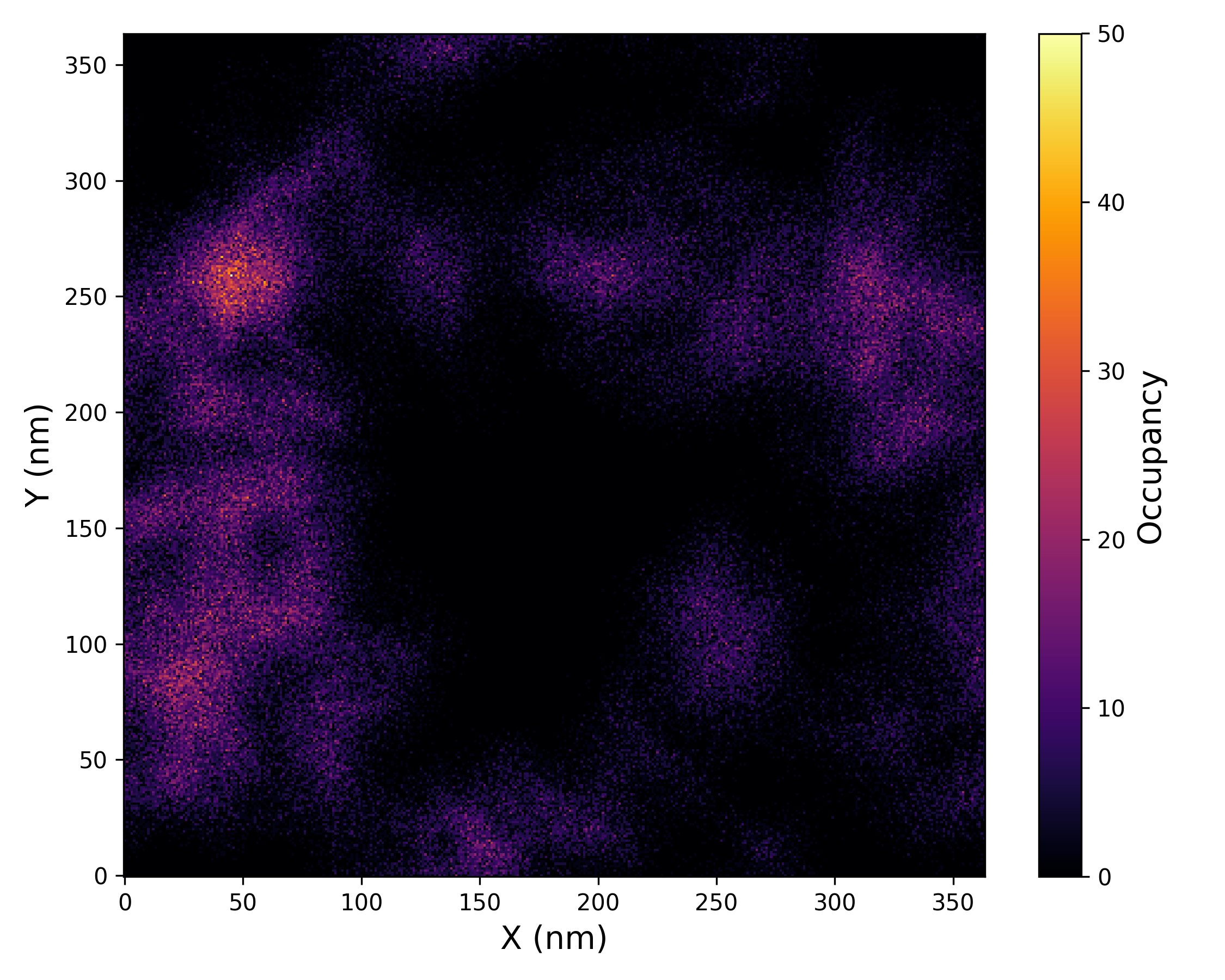
Interpretation guidance: This plot illustrates the relative density distribution of ligand atoms throughout the simulation. Regions with higher density values correspond to areas where the ligand spent more time, indicating preferred binding locations or stable interaction zones. Conversely, areas with lower density indicate less frequent ligand presence or greater positional variability.

Complete code

import numpy as np
import matplotlib.pyplot as plt
import os

def read_xpm(file_path):

"""
Reads a .xpm file and converts it into a 2D matrix of density values.

Parameters:
-----------
file_path : str
    Path to the .xpm file.

Returns:
--------
matrix : np.ndarray
    2D array of density values.
"""
with open(file_path, 'r') as f:
    lines = f.readlines()

# Keep only lines containing matrix content (i.e., starting with quotes)
lines = [l.strip() for l in lines if l.strip().startswith('"')]

# Parse the header line with matrix dimensions and color mapping details
header_line = lines[0].strip().strip('",')
width, height, ncolors, chars_per_pixel = map(int, header_line.split())

# Build the color symbol to value mapping
color_map = {}
for i in range(1, ncolors + 1):
    line = lines[i].strip().strip('",')
    symbol = line[:chars_per_pixel]
    color_map[symbol] = i - 1  # Assign unique integer values for plotting

# Convert the symbol matrix into a numeric matrix
matrix = []
for line in lines[ncolors + 1:]:
    line = line.strip().strip('",')
    row = [color_map[line[i:i+chars_per_pixel]] for i in range(0, len(line), chars_per_pixel)]
    matrix.append(row)

return np.array(matrix)

def plot_density(matrix, cmap='inferno', xlabel='X', ylabel='Y', title='',
             colorbar_label='Relative density', figsize=(6, 5),
             label_fontsize=12, save_path=None):

"""
Plots the ligand density matrix as a heatmap.

Parameters:
-----------
matrix : np.ndarray
    The ligand density matrix.
cmap : str
    Colormap used for the heatmap (e.g., 'inferno', 'jet').
xlabel, ylabel : str
    Axis labels for the plot.
title : str
    Title of the plot.
colorbar_label : str
    Label for the colorbar.
figsize : tuple
    Size of the figure (width, height in inches).
label_fontsize : int
    Font size used for all text labels.
save_path : str or None
    Path (without extension) where the plot will be saved.
"""
plt.figure(figsize=figsize)
img = plt.imshow(matrix, cmap=cmap, origin='lower', aspect='auto')
cbar = plt.colorbar(img)
cbar.set_label(colorbar_label, fontsize=label_fontsize)
plt.xlabel(xlabel, fontsize=label_fontsize)
plt.ylabel(ylabel, fontsize=label_fontsize)
plt.title(title, fontsize=label_fontsize + 2)
plt.tight_layout()

# Save plots in both PNG and TIFF formats
if save_path:
    base, _ = os.path.splitext(save_path)
    plt.savefig(f"{base}.png", dpi=300)
    plt.savefig(f"{base}.tiff", dpi=300)
    print(f"Figure saved as: {base}.png and {base}.tiff")

plt.show()

def ligand_density_analysis(xpm_file_path, output_path=None, plot=True,
                        cmap='inferno', xlabel='X', ylabel='Y',
                        title='', colorbar_label='Relative density',
                        figsize=(6, 5), label_fontsize=12):

"""
Main function to perform ligand density analysis from an .xpm file.

Parameters:
-----------
xpm_file_path : str
    Path to the input .xpm file.
output_path : str or None
    Base output path (without extension) to save figures.
plot : bool
    If True, displays the density plot.
cmap : str
    Colormap to use for the heatmap visualization.
xlabel, ylabel, title, colorbar_label : str
    Custom text for axis labels, title, and colorbar.
figsize : tuple
    Figure size in inches (width, height).
label_fontsize : int
    Font size for axis labels and title.

Returns:
--------
matrix : np.ndarray
    2D array representing the ligand density.
"""
matrix = read_xpm(xpm_file_path)
if plot:
    plot_density(matrix, cmap=cmap, xlabel=xlabel, ylabel=ylabel,
                 title=title, colorbar_label=colorbar_label,
                 figsize=figsize, label_fontsize=label_fontsize,
                 save_path=output_path)
return matrix