Principal Component Analysis

Overview

DynamiSpectra offers a robust and versatile analytical framework for performing principal component analysis (PCA) on molecular dynamics simulation data. Utilizing input in standardized .xvg file format, this module enables researchers to identify and characterize the dominant collective motions and conformational fluctuations of biomolecular systems.

Command line in GROMACS to generate .xvg files for the analysis:

gmx covar -f Simulation.xtc -s Simulation.tpr -o eingenvalues.xvg -v eingenvectors.trr -av average.pdb

gmx anaeig -v eingenvectors.trr -f Simulation.xtc -s Simulation.tpr -first 1 -last 2 -2d 2dproj.xvg

Note: PCA analysis requires the eigenvalues.xvg and 2dproj.xvg files.

def pca_analysis(pca_file_path, eigenval_path, output_folder,
             title="PCA", figsize=(7, 6), cmap="viridis",
             point_size=30, alpha=0.8):

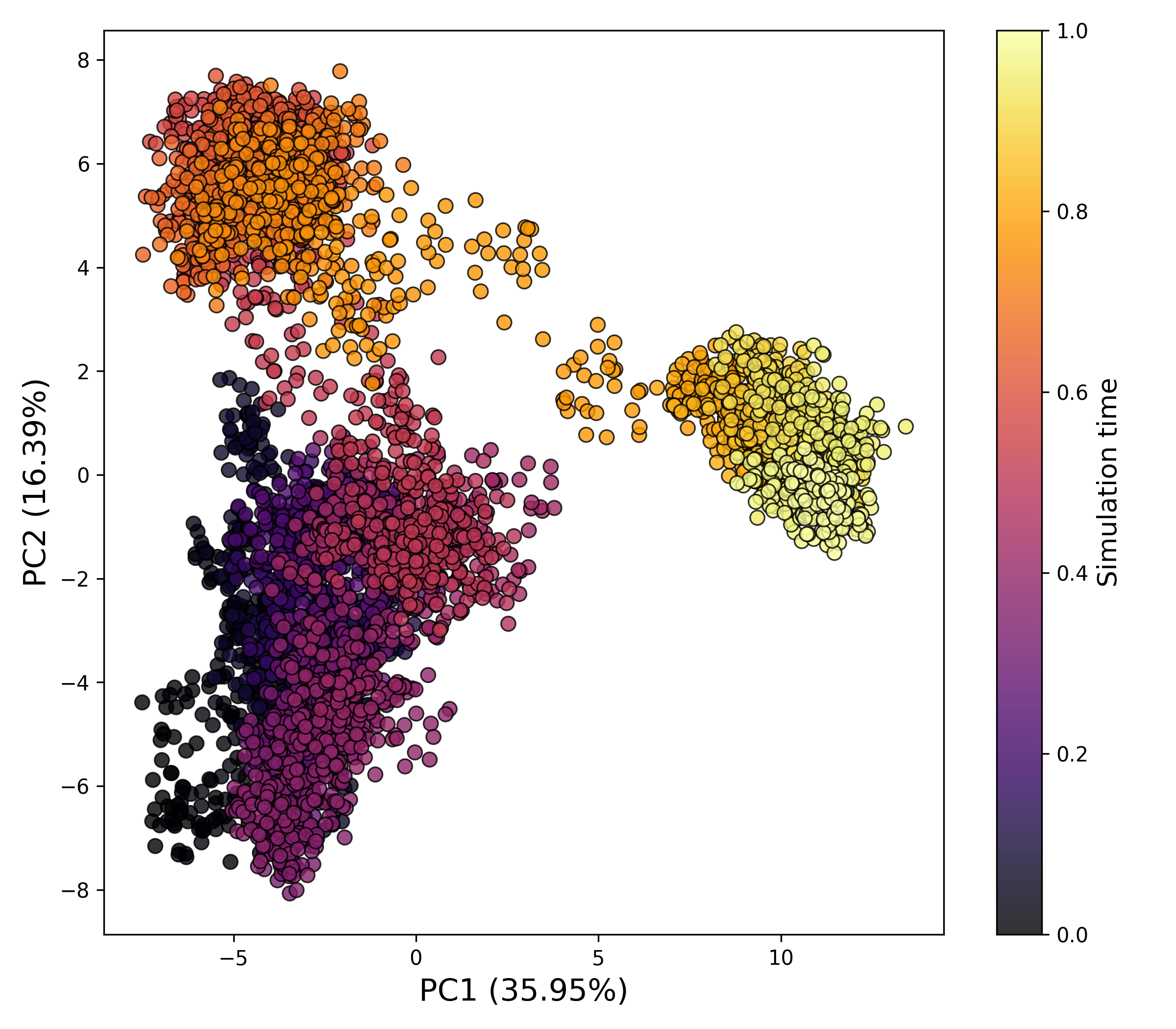
How to interpret: This plot illustrates the temporal or spatial distribution of motion projected along selected principal components (PCs). The first few PCs generally capture the most significant large-scale motions within the system. Dense clustering of data points may indicate stable conformational states, whereas more dispersed distributions suggest increased structural variability or transitions between different dynamic regimes.

Complete code

import numpy as np
import matplotlib.pyplot as plt
import os

def read_xvg(file_path):

"""
Reads PCA projection data from a .xvg file.

Parameters:
-----------
file_path : str
    Path to the .xvg file.

Returns:
--------
data : numpy.ndarray
    Array with PC1 and PC2 values.
"""
data = []
with open(file_path, "r") as file:
    for line in file:
        # Skip comment and metadata lines
        if not line.startswith(("#", "@")):
            values = line.split()
            data.append([float(values[0]), float(values[1])])
return np.array(data)

def read_eigenvalues(file_path):

"""
Reads eigenvalues from a .xvg file.

Parameters:
-----------
file_path : str
    Path to the eigenvalues .xvg file.

Returns:
--------
eigenvalues : numpy.ndarray
    Array of eigenvalues.
"""
eigenvalues = []
with open(file_path, "r") as file:
    for line in file:
        # Skip comment and metadata lines
        if not line.startswith(("#", "@")):
            eigenvalues.append(float(line.split()[1]))
return np.array(eigenvalues)

def plot_pca(pca_data, eigenvalues, output_folder, title="PCA",
         figsize=(7, 6), cmap="viridis", point_size=30, alpha=0.8):

"""
Generates a PCA scatter plot with customization options.

Parameters:
-----------
pca_data : numpy.ndarray
    Array with PC1 and PC2 values.
eigenvalues : numpy.ndarray
    Array of eigenvalues.
output_folder : str
    Folder to save the output figure.
title : str
    Title of the plot.
figsize : tuple
    Size of the figure (width, height).
cmap : str
    Color map for scatter points.
point_size : int or float
    Size of the scatter points.
alpha : float
    Transparency of the points (0 to 1).
"""
total_variance = np.sum(eigenvalues)
pc1_var = (eigenvalues[0] / total_variance) * 100
pc2_var = (eigenvalues[1] / total_variance) * 100

plt.figure(figsize=figsize)
scatter = plt.scatter(
    pca_data[:, 0], pca_data[:, 1],
    c=np.linspace(0, 1, len(pca_data)),  # Color by simulation time
    cmap=cmap,
    s=point_size,
    alpha=alpha,
    edgecolors='k',
    linewidths=0.8
)

plt.xlabel(f"PC1 ({pc1_var:.2f}%)", fontsize=12)
plt.ylabel(f"PC2 ({pc2_var:.2f}%)", fontsize=12)
plt.title(title, fontsize=14)
plt.colorbar(scatter, label="Simulation time")

plt.grid(False)
plt.tight_layout()

# Create the output folder if it does not exist
os.makedirs(output_folder, exist_ok=True)

# Save the figure in high resolution
plt.savefig(os.path.join(output_folder, 'pca_plot.png'), dpi=300)
plt.show()

def pca_analysis(pca_file_path, eigenval_path, output_folder,
             title="PCA", figsize=(7, 6), cmap="viridis",
             point_size=30, alpha=0.8):

"""
Runs PCA analysis and generates the scatter plot.

Parameters:
-----------
pca_file_path : str
    Path to the PCA projection file (usually 'pca_proj.xvg').
eigenval_path : str
    Path to the eigenvalues file (usually 'eigenval.xvg').
output_folder : str
    Folder to save the output plot.
title : str
    Plot title.
figsize : tuple
    Size of the figure.
cmap : str
    Colormap for the scatter plot.
point_size : int or float
    Size of scatter points.
alpha : float
    Transparency of scatter points.
"""
pca_data = read_xvg(pca_file_path)
eigenvalues = read_eigenvalues(eigenval_path)
plot_pca(pca_data, eigenvalues, output_folder, title, figsize, cmap, point_size, alpha)