System Density
Overview
DynamiSpectra offers a comprehensive analytical framework to evaluate the density distribution within molecular systems during molecular dynamics simulations, utilizing input data in .xvg file format. This analysis enables detailed insights into the spatial arrangement and concentration of particles in the system.
The software’s graphical interface allows users to visualize the average density profiles derived from multiple simulation replicates, with the corresponding standard deviation depicted as a shaded region to represent variability. Additionally, DynamiSpectra supports the analysis of individual simulation replicas, enabling plots to be generated from single datasets when multiple replicates are not available or not required.
Command line in GROMACS to generate .xvg files for the analysis:
gmx energy -f Simulation.edr -o Density.xvg
def density_analysis(output_folder, *simulation_file_groups, density_config=None, distribution_config=None)
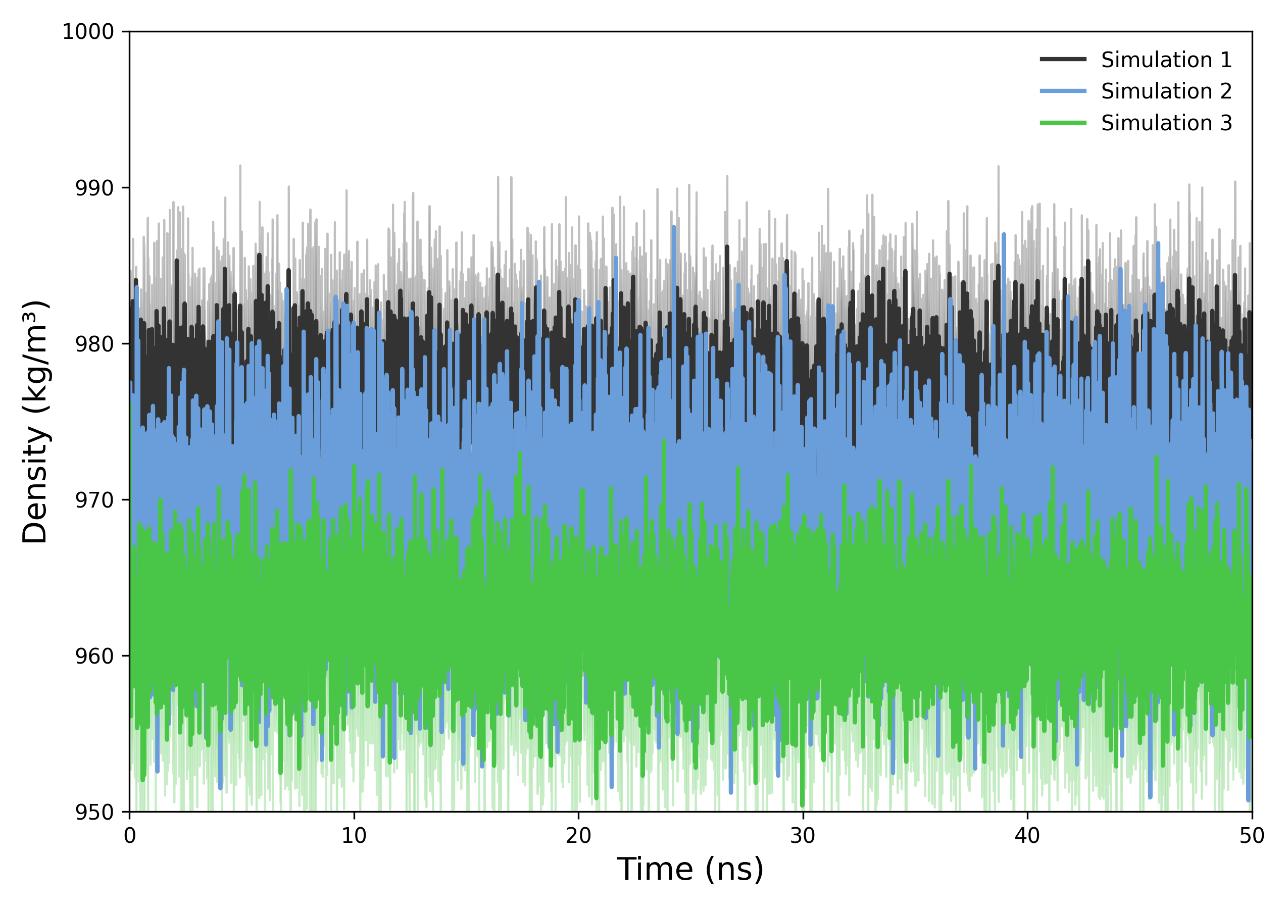
Interpretation guidance: The resulting plots illustrate the temporal evolution of system density. A consistent profile indicates stable particle distribution throughout the simulation, while significant fluctuations may reflect structural rearrangements, phase transitions, or other dynamic processes affecting system compactness or organization of the system.
def plot_density_distribution(results, output_folder, config=None)
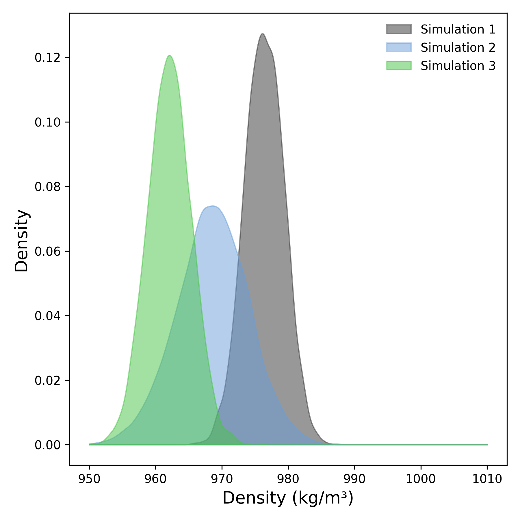
Interpretation guidance: This plot represents the density distribution derived from the temporal profile of system density. Peaks in the distribution indicate regions of higher particle concentration within the system. Broader peaks suggest a more heterogeneous or variable distribution, whereas sharper, well-defined peaks correspond to stable and consistent density regions throughout the simulation.
Complete code
import numpy as np
import matplotlib.pyplot as plt
from scipy.stats import gaussian_kde
import os
def read_density(file):
"""
Reads density data from a .xvg file and returns time (in ns) and density values.
"""
try:
    times = []
    densities = []
    with open(file, 'r') as f:
        for line in f:
            # Skip comments and formatting lines
            if line.startswith(('#', '@', ';')) or line.strip() == '':
                continue
            try:
                values = line.split()
                if len(values) >= 2:
                    # Extract time (ps) and density, then convert time to ns
                    time_ps, density_val = map(float, values[:2])
                    times.append(time_ps / 1000.0)
                    densities.append(density_val)
            except ValueError:
                # Ignore lines that cannot be converted to floats
                continue
    # Raise error if no valid data found
    if len(times) == 0 or len(densities) == 0:
        raise ValueError(f"File {file} does not contain valid data.")
    return np.array(times), np.array(densities)
except Exception as e:
    print(f"Error reading file {file}: {e}")
    return None, None
def check_simulation_times(*time_arrays):
"""
Checks if all provided time arrays are consistent (equal within tolerance).
Raises an error if any discrepancy is found.
"""
for i in range(1, len(time_arrays)):
    if not np.allclose(time_arrays[0], time_arrays[i]):
        raise ValueError(f"Simulation times do not match between file 1 and file {i+1}")
def plot_density(results, output_folder, config=None):
"""
Plots mean density over time with shaded standard deviation area for multiple simulations.

Parameters:
-----------
results : list of tuples
    Each tuple contains (time_array, mean_density, std_density).
output_folder : str
    Path where plots will be saved.
config : dict, optional
    Dictionary with plot customization (colors, labels, figure size, etc.).
"""
plt.figure(figsize=config.get('figsize', (9, 6)))
for idx, (time, mean, std) in enumerate(results):
    # Set label and color for each simulation
    label = config['labels'][idx] if config and 'labels' in config else f'Simulation {idx+1}'
    color = config['colors'][idx] if config and 'colors' in config else None
    alpha = config.get('alpha', 0.2)

    # Plot mean density line and shaded std deviation area
    plt.plot(time, mean, label=label, color=color, linewidth=2)
    plt.fill_between(time, mean - std, mean + std, color=color, alpha=alpha)

# Set plot labels and legend
plt.xlabel(config.get('xlabel', 'Time (ns)'), fontsize=config.get('label_fontsize', 12))
plt.ylabel(config.get('ylabel', 'Density (kg/m³)'), fontsize=config.get('label_fontsize', 12))
plt.legend(frameon=False, loc='upper right', fontsize=10)
plt.tick_params(axis='both', which='major', labelsize=10)

# Set axis limits dynamically if specified
max_time = max([np.max(time) for time, _, _ in results])
plt.xlim(0, max_time)
if 'ylim' in config:
    plt.ylim(config['ylim'])

# Save plots to output folder
plt.tight_layout()
os.makedirs(output_folder, exist_ok=True)
plt.savefig(os.path.join(output_folder, 'density_plot.tiff'), dpi=300)
plt.savefig(os.path.join(output_folder, 'density_plot.png'), dpi=300)
plt.show()
def plot_density_distribution(results, output_folder, config=None):
"""
Plots KDE-based smooth distributions of mean density values for multiple simulations.

Parameters:
-----------
results : list of tuples
    Each tuple contains (time_array, mean_density, std_density).
    Only mean_density is used for KDE estimation.
output_folder : str
    Path where plots will be saved.
config : dict, optional
    Dictionary with plot customization (colors, labels, figure size, etc.).
"""
plt.figure(figsize=config.get('figsize', (6, 6)))
for idx, (_, mean, _) in enumerate(results):
    # Kernel Density Estimation for smooth density distribution
    kde = gaussian_kde(mean)
    x_min = config.get('x_min', np.min(mean))
    x_max = config.get('x_max', np.max(mean))
    x_vals = np.linspace(x_min, x_max, 1000)

    # Plot KDE fill for each simulation
    label = config['labels'][idx] if config and 'labels' in config else f'Simulation {idx+1}'
    color = config['colors'][idx] if config and 'colors' in config else None
    alpha = config.get('alpha', 0.5)
    plt.fill_between(x_vals, kde(x_vals), color=color, alpha=alpha, label=label)

# Set plot labels and legend
plt.xlabel(config.get('xlabel', 'Density (kg/m³)'), fontsize=config.get('label_fontsize', 12))
plt.ylabel(config.get('ylabel', 'Density'), fontsize=config.get('label_fontsize', 12))
plt.legend(frameon=False, loc='upper right', fontsize=10)
plt.tight_layout()

# Save KDE plots to output folder
plt.savefig(os.path.join(output_folder, 'density_distribution.tiff'), dpi=300)
plt.savefig(os.path.join(output_folder, 'density_distribution.png'), dpi=300)
plt.show()
def density_analysis(output_folder, *simulation_file_groups, density_config=None, distribution_config=None):
"""
Processes multiple simulation groups with density replicate files,
computes mean and standard deviation, and generates plots.

Parameters:
-----------
output_folder : str
    Directory path where plots will be saved.
*simulation_file_groups : list of lists
    Each argument is a list of file paths for replicate density data of one simulation.
density_config : dict, optional
    Configuration dictionary for time series density plot.
distribution_config : dict, optional
    Configuration dictionary for density distribution (KDE) plot.
"""
def process_group(file_paths):
    times = []
    densities = []
    for file in file_paths:
        # Read density data from each replicate file
        time, density_val = read_density(file)
        times.append(time)
        densities.append(density_val)

    # Check that all replicates have consistent time points
    check_simulation_times(*times)

    # Calculate mean and standard deviation across replicates
    density_array = np.array(densities)
    mean_density = np.mean(density_array, axis=0)
    std_density = np.std(density_array, axis=0)
    return times[0], mean_density, std_density

results = []
for group in simulation_file_groups:
    if group:
        time, mean, std = process_group(group)
        results.append((time, mean, std))

# Generate plots if at least one simulation group is processed
if len(results) >= 1:
    plot_density(results, output_folder, config=density_config)
    plot_density_distribution(results, output_folder, config=distribution_config)
else:
    raise ValueError("At least one simulation group with replicate files is required.")