Protein-Ligand Minimal Distance
Overview
DynamiSpectra provides a rigorous and versatile analytical framework designed to quantify and monitor the dynamic distances between protein and ligand molecules throughout the course of molecular dynamics simulations. Utilizing input data in standardized .xvg file format, this module enables researchers to precisely evaluate intermolecular spatial relationships, which are critical for understanding binding affinity, conformational changes, and interaction stability.
This analysis offers a comprehensive perspective on how the proximity between the protein and ligand evolves over time, allowing identification of transient interactions, stable binding modes, or dissociation events. By incorporating multiple simulation replicates, DynamiSpectra calculates averaged distance profiles along with corresponding measures of variability, such as standard deviation, to provide statistically meaningful insights. Additionally, the software accommodates the evaluation of individual simulation replicas, enabling flexible application where replicate data may be limited or unnecessary.
Command line in GROMACS to generate .xvg files for the analysis:
gmx mindist -f Simulation.xtc -s Simulation.tpr -n index.ndx -od Distance.xvg -d 0.35
def distance_analysis(output_folder, *simulation_file_groups, distance_config=None, density_config=None)
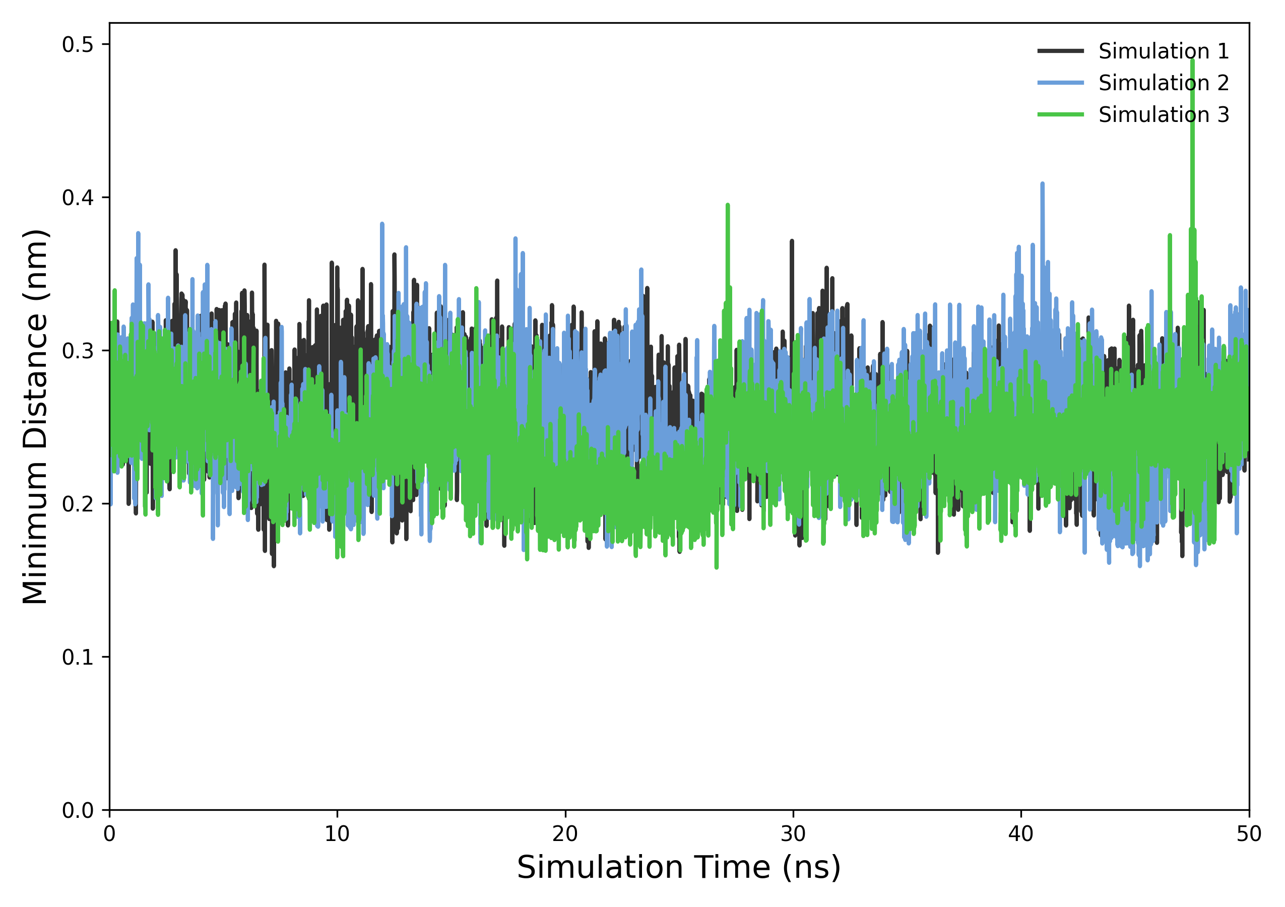
Interpretation guidance: The resulting plots depict the temporal evolution of the minimal distances between protein and ligand atoms. Consistently low minimal distances suggest stable close contacts or binding, while significant increases or fluctuations may indicate conformational changes, ligand dissociation, or transient interactions
def plot_distance_density(results, output_folder, config=None)
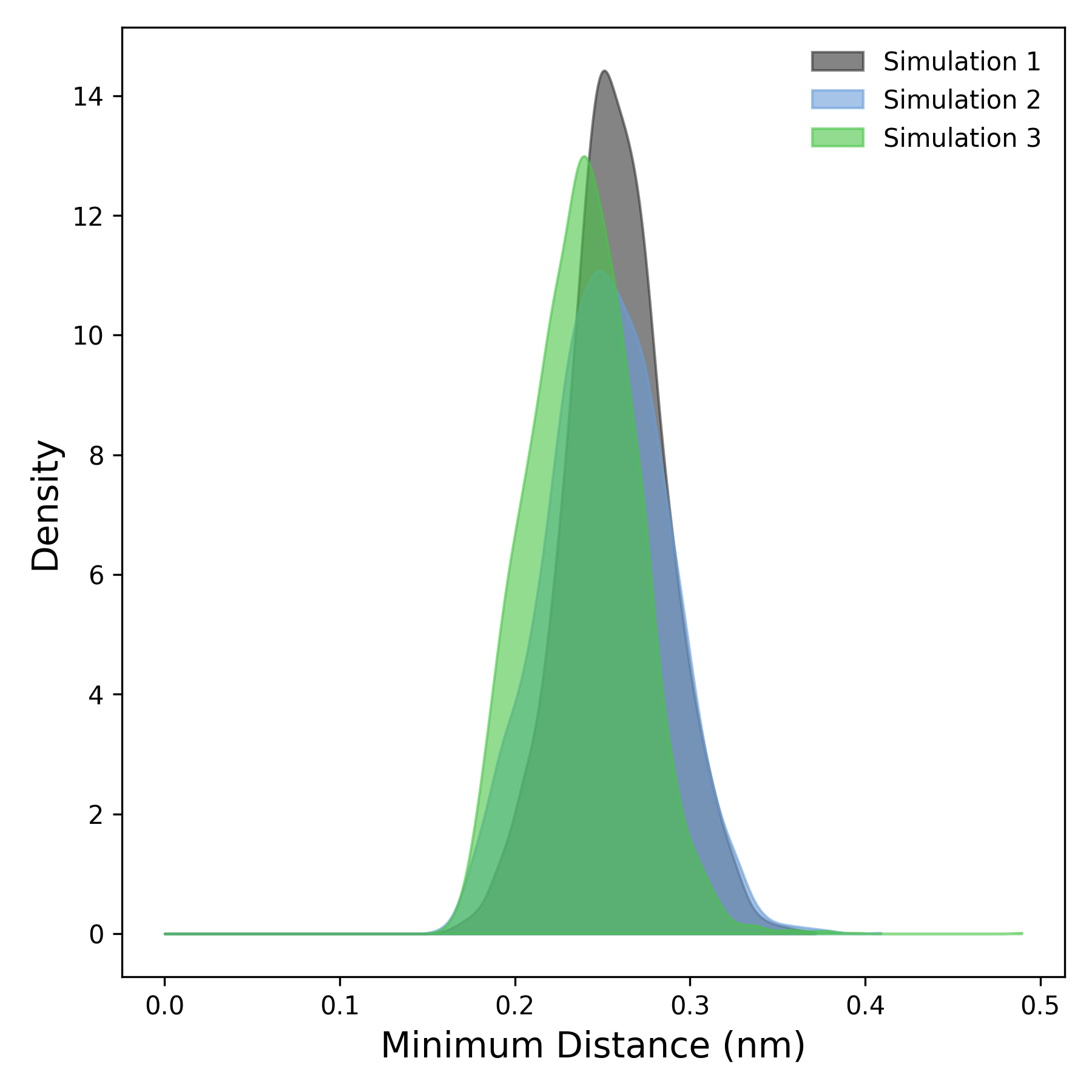
Interpretation guidance: This plot illustrates the density distribution derived from the temporal profile of the minimal distance between protein and ligand. Peaks in the distribution signify regions where the minimal distances occur more frequently, indicating preferred interaction distances. Broader peaks suggest a more variable and heterogeneous range of distances, while sharper, well-defined peaks reflect stable and consistent interaction proximities throughout the simulation.
Complete code
import numpy as np
import matplotlib.pyplot as plt
from scipy.stats import gaussian_kde
import os
def read_distance(file):
"""
Reads minimum distance data from a .xvg file.
Skips header lines and extracts time (in ns) and distance values.

Parameters:
-----------
file : str
    Path to the .xvg file

Returns:
--------
times : np.ndarray
    Array of time points in nanoseconds.
distances : np.ndarray
    Array of minimum distances at each time point.
"""
try:
    times = []
    distances = []
    with open(file, 'r') as f:
        for line in f:
            # Skip comments and empty lines
            if line.startswith(('#', '@', ';')) or line.strip() == '':
                continue
            try:
                values = line.split()
                if len(values) >= 2:
                    time_ps, dist_val = map(float, values[:2])
                    times.append(time_ps / 1000.0)  # Convert from ps to ns
                    distances.append(dist_val)
            except ValueError:
                # Ignore lines that cannot be converted to floats
                continue

    # Check if data was read correctly
    if len(times) == 0 or len(distances) == 0:
        raise ValueError(f"File {file} does not contain valid data.")

    return np.array(times), np.array(distances)

except Exception as e:
    print(f"Error reading file {file}: {e}")
    return None, None
def check_simulation_times(*time_arrays):
"""
Checks if all simulation time arrays are consistent (equal).
Raises an error if times do not match to avoid misaligned averaging.
"""
for i in range(1, len(time_arrays)):
    if not np.allclose(time_arrays[0], time_arrays[i]):
        raise ValueError(f"Simulation times do not match between file 1 and file {i+1}")
def plot_distance(results, output_folder, config=None):
"""
Plots the mean minimum distance over time with shaded std deviation.

Parameters:
-----------
results : list of tuples
    Each tuple is (time_array, mean_distance, std_distance) for one simulation group.
output_folder : str
    Folder path to save the plots.
config : dict, optional
    Plot configuration dictionary (colors, labels, axis labels, etc.)
"""
plt.figure(figsize=config.get('figsize', (9, 6)))

# Plot mean ± std for each simulation group
for idx, (time, mean, std) in enumerate(results):
    label = config['labels'][idx] if config and 'labels' in config else f'Simulation {idx+1}'
    color = config['colors'][idx] if config and 'colors' in config else None
    alpha = config.get('alpha', 0.2)
    plt.plot(time, mean, label=label, color=color, linewidth=2)
    plt.fill_between(time, mean - std, mean + std, color=color, alpha=alpha)

plt.xlabel(config.get('xlabel', 'Time (ns)'), fontsize=config.get('label_fontsize', 12))
plt.ylabel(config.get('ylabel', 'Minimum Distance (nm)'), fontsize=config.get('label_fontsize', 12))
plt.legend(frameon=False, loc='upper right', fontsize=10)
plt.tick_params(axis='both', which='major', labelsize=10)

# Dynamically set x and y axis limits to start at 0 and cover data range with margin
max_time = max([np.max(time) for time, _, _ in results])
max_val = max([np.max(mean + std) for _, mean, std in results])
plt.xlim(0, max_time)
plt.ylim(0, max_val * 1.05)  # Add 5% margin above max

plt.tight_layout()

# Create output folder if it doesn't exist
os.makedirs(output_folder, exist_ok=True)

# Save plots in TIFF and PNG formats
plt.savefig(os.path.join(output_folder, 'distance_plot.tiff'), dpi=300)
plt.savefig(os.path.join(output_folder, 'distance_plot.png'), dpi=300)

plt.show()
def plot_distance_density(results, output_folder, config=None):
"""
Plots kernel density estimates of the minimum distance distributions.

Parameters:
-----------
results : list of tuples
    Each tuple is (time_array, mean_distance, std_distance).
    Only the mean_distance array is used here for density estimation.
output_folder : str
    Folder path to save the density plots.
config : dict, optional
    Plot configuration dictionary.
"""
plt.figure(figsize=config.get('figsize', (6, 6)))

# Plot KDE for each simulation group's mean distance values
for idx, (_, mean, _) in enumerate(results):
    kde = gaussian_kde(mean)
    x_vals = np.linspace(0, max(mean), 1000)
    label = config['labels'][idx] if config and 'labels' in config else f'Simulation {idx+1}'
    color = config['colors'][idx] if config and 'colors' in config else None
    alpha = config.get('alpha', 0.5)
    plt.fill_between(x_vals, kde(x_vals), color=color, alpha=alpha, label=label)

plt.xlabel(config.get('xlabel', 'Minimum Distance (nm)'), fontsize=config.get('label_fontsize', 12))
plt.ylabel(config.get('ylabel', 'Density'), fontsize=config.get('label_fontsize', 12))
plt.legend(frameon=False, loc='upper right', fontsize=10)
plt.tight_layout()

# Save density plots
plt.savefig(os.path.join(output_folder, 'distance_density.tiff'), dpi=300)
plt.savefig(os.path.join(output_folder, 'distance_density.png'), dpi=300)

plt.show()
def distance_analysis(output_folder, *simulation_file_groups, distance_config=None, density_config=None):
"""
Main function to process multiple simulation groups and generate minimum distance plots.

Parameters:
-----------
output_folder : str
    Directory where the plots will be saved.
*simulation_file_groups : list of lists
    Each element is a list of file paths for replicates of a simulation group.
distance_config : dict, optional
    Configuration for the distance vs time plot.
density_config : dict, optional
    Configuration for the density plot.
"""
def process_group(file_paths):
    times = []
    distances = []
    for file in file_paths:
        time, dist_val = read_distance(file)
        times.append(time)
        distances.append(dist_val)
    check_simulation_times(*times)
    mean_distance = np.mean(distances, axis=0)
    std_distance = np.std(distances, axis=0)
    return times[0], mean_distance, std_distance

results = []
for group in simulation_file_groups:
    if group:
        time, mean, std = process_group(group)
        results.append((time, mean, std))

if len(results) >= 1:
    plot_distance(results, output_folder, config=distance_config)
    plot_distance_density(results, output_folder, config=density_config)
else:
    raise ValueError("At least one simulation group is required.")