Solvent Accessible Surface Area
Overview
DynamiSpectra provides a comprehensive Solvent Accessible Surface Area (SASA) analysis module for molecular dynamics simulations. This module supports both individual replica analysis and the calculation of statistical metrics (mean and standard deviation) across multiple simulation replicas. The resulting plots display the average SASA over time with shaded regions representing the variability across replicates. This enables users to assess trends in solvent exposure and compare results across different conditions or systems.
Command line in GROMACS to generate .xvg files for the analysis:
gmx sasa -s Simulation.tpr -f Simulation.xtc -o sasa_simulation.xvg -probe 0.14
def sasa_analysis(output_folder, *simulation_files_groups, sasa_config=None, density_config=None)
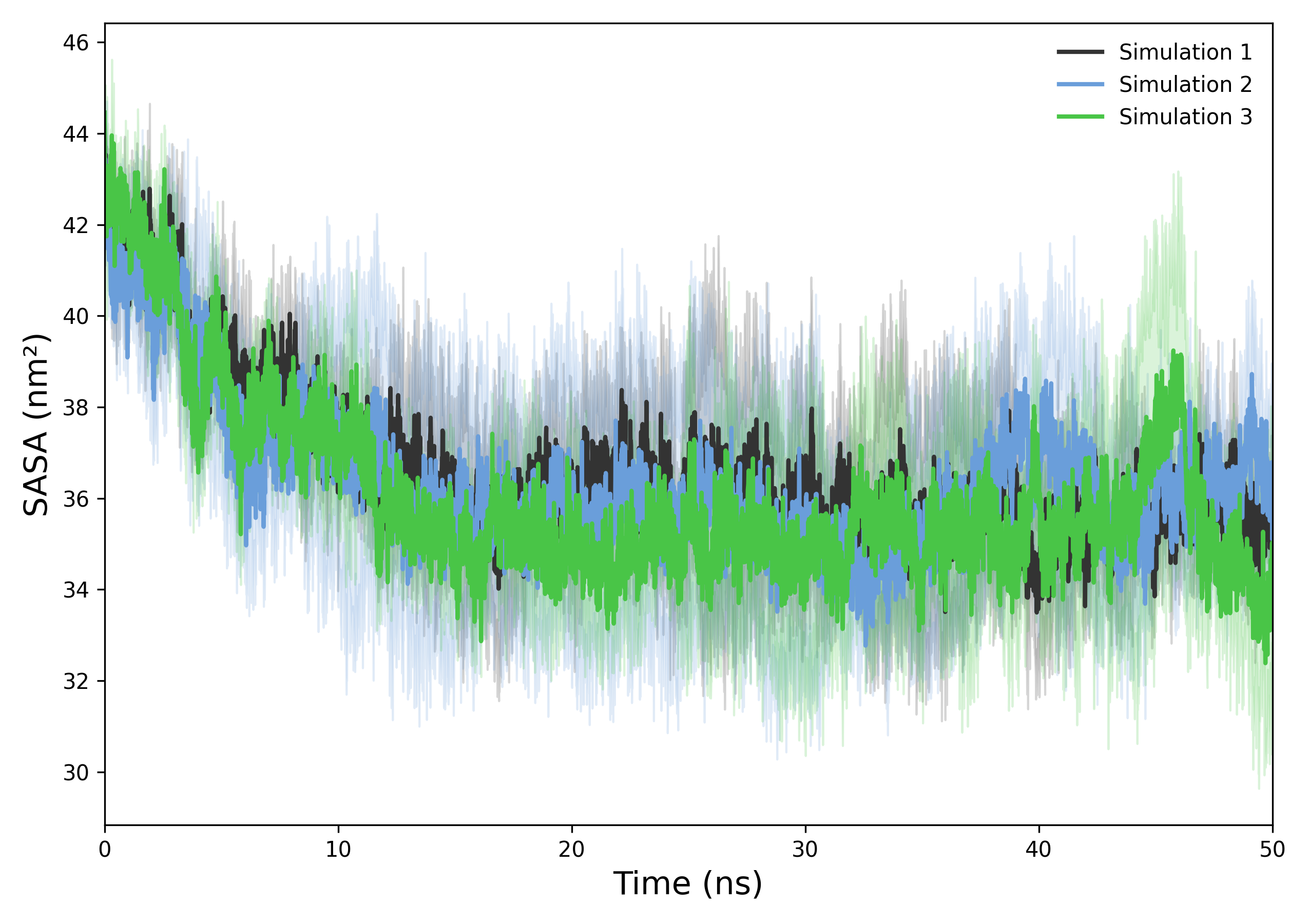
Interpretation guidence This graph shows the SASA over time, with the mean and standard deviation across replicas. A stable SASA indicates that the system maintains a consistent solvent-exposed surface area. Sudden increases may reflect unfolding or expansion, while decreases can suggest compaction or structural collapse. Monitoring SASA trends helps reveal conformational changes during the simulation.
def plot_density(means_list, output_folder, config)
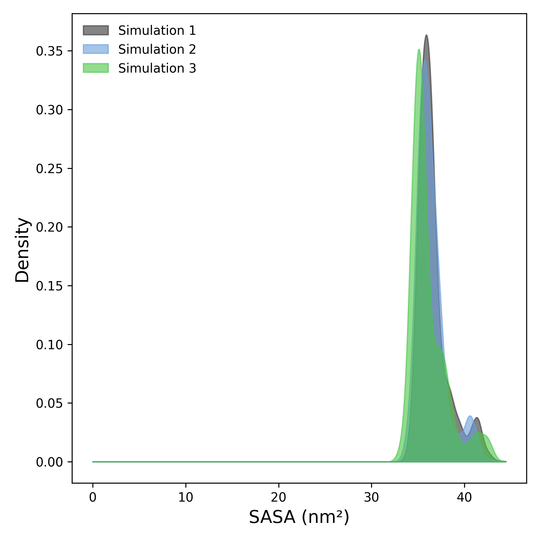
Interpretation guidence: This graph shows the probability distribution of SASA values across the simulation. Peaks indicate the most frequently sampled solvent-accessible areas. Narrow, sharp peaks suggest structural stability, while broader distributions reflect greater conformational variability. Comparing curves across simulations can reveal differences in surface exposure behavior.
Complete code
import numpy as np
import matplotlib.pyplot as plt
from scipy.stats import gaussian_kde
import os
def read_sasa(file):
"""
Reads SASA data from a GROMACS .xvg file.
Converts time from ps to ns.
Returns numpy arrays of time and SASA.
"""
try:
    print(f"Reading file: {file}")
    times, sasas = [], []
    with open(file, 'r') as f:
        for line in f:
            # Skip comments and empty lines
            if line.startswith(('#', '@', ';')) or line.strip() == '':
                continue
            try:
                values = line.split()
                if len(values) >= 2:
                    time, sasa = map(float, values[:2])
                    times.append(time / 1000)  # convert ps to ns
                    sasas.append(sasa)
            except ValueError:
                print(f"Error processing line: {line.strip()}")
                continue
    if len(times) == 0 or len(sasas) == 0:
        raise ValueError(f"File {file} does not contain valid data.")
    return np.array(times), np.array(sasas)
except Exception as e:
    print(f"Error reading file {file}: {e}")
    return None, None
def check_simulation_times(*time_arrays):
"""
Checks if all provided time arrays are approximately equal.
Raises ValueError if any mismatch is found.
"""
for i in range(1, len(time_arrays)):
    if not np.allclose(time_arrays[0], time_arrays[i]):
        raise ValueError(f"Simulation times do not match between file 1 and file {i+1}")
def plot_sasa(times_list, means_list, stds_list, output_folder, config):
"""
Plots SASA time series with mean ± std deviation shaded regions.
Accepts dynamic number of simulation groups.
"""
labels = config.get('labels', [f'Simulation {i+1}' for i in range(len(times_list))])
colors = config.get('colors', ['#333333', '#6A9EDA', '#54b36a', '#e377c2', '#8c564b', '#17becf'])
alpha = config.get('alpha', 0.2)
figsize = config.get('figsize', (7, 6))
xlabel = config.get('xlabel', 'Time (ns)')
ylabel = config.get('ylabel', 'SASA (nm²)')
label_fontsize = config.get('label_fontsize', 12)
xlim = config.get('xlim', None)
ylim = config.get('ylim', None)

plt.figure(figsize=figsize)

for i, (t, m, s) in enumerate(zip(times_list, means_list, stds_list)):
    if t is not None:
        color = colors[i % len(colors)]
        label = labels[i] if i < len(labels) else f'Simulation {i+1}'
        plt.plot(t, m, label=label, color=color, linewidth=2)
        plt.fill_between(t, m - s, m + s, color=color, alpha=alpha)

plt.xlabel(xlabel, fontsize=label_fontsize)
plt.ylabel(ylabel, fontsize=label_fontsize)
plt.legend(frameon=False, loc='upper right', fontsize=10)
plt.tick_params(axis='both', which='major', labelsize=10)

if xlim:
    plt.xlim(xlim)
else:
    all_times = [t for t in times_list if t is not None]
    plt.xlim(0, max([t[-1] for t in all_times]))

if ylim:
    plt.ylim(ylim)

plt.tight_layout()
os.makedirs(output_folder, exist_ok=True)
plt.savefig(os.path.join(output_folder, 'sasa_plot.tiff'), format='tiff', dpi=300)
plt.savefig(os.path.join(output_folder, 'sasa_plot.png'), format='png', dpi=300)
plt.show()
def plot_density(means_list, output_folder, config):
"""
Plots KDE density of SASA distributions for each simulation group.
Accepts dynamic number of simulation groups.
"""
labels = config.get('labels', [f'Simulation {i+1}' for i in range(len(means_list))])
colors = config.get('colors', ['#333333', '#6A9EDA', '#54b36a', '#e377c2', '#8c564b', '#17becf'])
alpha = config.get('alpha', 0.5)
figsize = config.get('figsize', (6, 6))
xlabel = config.get('xlabel', 'SASA (nm²)')
ylabel = config.get('ylabel', 'Density')
label_fontsize = config.get('label_fontsize', 12)
xlim = config.get('xlim', None)
ylim = config.get('ylim', None)

plt.figure(figsize=figsize)

for i, m in enumerate(means_list):
    if m is not None:
        color = colors[i % len(colors)]
        label = labels[i] if i < len(labels) else f'Simulation {i+1}'
        kde = gaussian_kde(m)
        x = np.linspace(0, max(m), 1000)
        plt.fill_between(x, kde(x), color=color, alpha=alpha, label=label)

plt.xlabel(xlabel, fontsize=label_fontsize)
plt.ylabel(ylabel, fontsize=label_fontsize)
plt.legend(frameon=False, loc='upper left', fontsize=10)
plt.tick_params(axis='both', which='major', labelsize=10)

if xlim:
    plt.xlim(xlim)
if ylim:
    plt.ylim(ylim)

plt.tight_layout()
os.makedirs(output_folder, exist_ok=True)
plt.savefig(os.path.join(output_folder, 'density_plot.tiff'), format='tiff', dpi=300)
plt.savefig(os.path.join(output_folder, 'density_plot.png'), format='png', dpi=300)
plt.show()
def sasa_analysis(output_folder, *simulation_files_groups, sasa_config=None, density_config=None):
"""
Main function to analyze SASA from multiple simulation groups and replicas.
Each group is a list of replicate file paths.
Computes mean ± std and generates plots.
"""
if sasa_config is None:
    sasa_config = {}
if density_config is None:
    density_config = {}

def process_group(file_paths):
    """
    Processes one simulation group (multiple replicas).
    Reads SASA data, checks time consistency, returns mean and std.
    """
    times, sasas = [], []
    for file in file_paths:
        time, sasa = read_sasa(file)
        if time is None or sasa is None:
            raise ValueError(f"Error reading file: {file}.")
        times.append(time)
        sasas.append(sasa)
    check_simulation_times(*times)
    return times[0], np.mean(sasas, axis=0), np.std(sasas, axis=0)

results = []
for group in simulation_files_groups:
    if group:
        time, mean, std = process_group(group)
        results.append((time, mean, std))

if not results:
    raise ValueError("You must provide at least one group of simulation files.")

# Unpack results dynamically for plotting
times_list, means_list, stds_list = zip(*results)

# Plot time series for all groups
plot_sasa(times_list, means_list, stds_list, output_folder, sasa_config)
# Plot KDE densities for all groups
plot_density(means_list, output_folder, density_config)